Paths & Curves
Some days ago I was fiddling with some Lua code, intending to achieve a splash/boot screen inspired to the one developed by Nintendo for the Game Boy. A single-line text entering from the top of the screen and scrolling down until it reaches the centre of it. Once on the final position, a jingle is played.
Notwithstanding being a very basic task, it offers the opportunity for uncovering some interesting code. The most naïve approach requires very little code and it would certainly work. With some additional effort, we can develop some interesting and general code that can be reused in many other circumstances. The most interesting part is how the text is moved through the screen, that is the path it follows. Rather than coding the path movement inside the Message object we are better off creating a Path object that implements it and that can be used by the former.
What kind of paths do we need to implement? We’d like the path to be a sequence of segments. Segments are going to be linear, but curved ones can be useful. A very straightforward way to implement this is by means of Bézier curves. I’m not going to describe them here (I suggest you follow the link to Wikipedia and read there), let’s just say they are very appealing since by simple playing with the curve order one can go from linear to smooth curves.
Let’s dive in some code and seem them in action.
function linear_bezier(p0, p1, t)
    local x = (1 - t) * p0[1] + t * p1[1]
    local y = (1 - t) * p0[2] + t * p1[2]
    return x, y
end

function quadratic_bezier(p0, p1, p2, t)
    local x = (1 - t) * (1 - t) * p0[1] + 2 * (1 - t) * t * p1[1] + t * t * p2[1]
    local y = (1 - t) * (1 - t) * p0[2] + 2 * (1 - t) * t * p1[2] + t * t * p2[2]
    return x, y
end

function cubic_bezier(p0, p1, p2, p3, t)
    local x = (1 - t) * (1 - t) * p0[1] + 2 * (1 - t) * t * p1[1] + t * t * p2[1]
    local y = (1 - t) * (1 - t) * p0[2] + 2 * (1 - t) * t * p1[2] + t * t * p2[2]
    return x, y
end
Easy, uh? An unpretentious and straightforward translation to Lua of the Bernstein polynomial representing the Bézier curves.
Another way to accomplish this is with the De Casteljau’s algorithm, which is in layman’s word a recursive lerp between pairs of control points.
function lerp(a, b, t)
    return (1 - t) * a + t * b
end

function linear_bezier(p0, p1, t)
    return lerp(p0[1], p1[1], t), lerp(p0[2], p1[2], t)
end

function quadratic_bezier(p0, p1, p2, t)
    local p01 = { linear_bezier(p0, p1, t) }
    local p12 = { linear_bezier(p1, p2, t) }
    return linear_bezier(p01, p12, t)
end

function cubic_bezier(p0, p1, p2, p3, t)
    local p01 = { linear_bezier(p0, p1, t) }
    local p12 = { linear_bezier(p1, p2, t) }
    local p23 = { linear_bezier(p2, p3, t) }
    local p012 = { linear_bezier(p01, p12, t) }
    local p123 = { linear_bezier(p12, p23, t) }
    return linear_bezier(p012, p123, t)
end
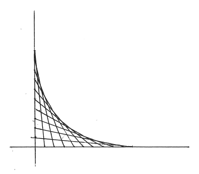
The visual representation of the De Casteljau algorithm is what many children learn as string art.
Refining
Both codes are presumably going to give bad performance: no precalculations, a lot of table accesses, creations, and ample use of function calls. There’s plenty of rooms for optimizations. Wait, wait, wait! We all know that premature optimization is evil, but we can be confident to write some elegant and efficient code. Here’s a brief list of changes we can apply:
- the control points can be passed as a table (i.e. vector) for a more compact function signature,
- there’s no need to pass the control points every time,
- we can avoid the recursion if we limit ourselves to some reasonable Bézier curve order (e.g. cubic) and use the Bernstein polynomial,
- some repeated math operations can be pre-computed and reused to save time, and
- closures and table unpacking can be used for faster access to functions/variables.
The final resulting code (warning, spoiler ahead since this is going to be the implementation that we’ll pick as “most performant”).
-- The function *compiles* a Bézier curve evaluator, given the control points
-- (as two-element arrays). The aim of this function is to avoid passing the
-- control-control_points at each evaluation.
--
-- It supports linear, quadratic, and cubic Bézier's curves. The evaluators are
-- the following (with `u = 1 - t`)
--
-- B1(p0, p1, t) = u*p0 + t*p1
-- B2(p0, p1, p2, t) = u*u*p0 + 2*t*u*p1 + t*t*p2
-- B3(p0, p1, p2, p3, t) = u*u*u*p0 + 3*u*u*t*p1 + 3*u*t*t*p2 + t*t*t*p3
local function compile_bezier(control_points)
  local n = #control_points
  if n == 4 then
    local p0, p1, p2, p3 = unpack(control_points)
    local p0x, p0y = unpack(p0)
    local p1x, p1y = unpack(p1)
    local p2x, p2y = unpack(p2)
    local p3x, p3y = unpack(p3)
    return function(t)
        local u = 1 - t
        local uu = u * u
        local tt = t * t
        local a = uu * u
        local b = 3 * uu * t
        local c = 3 * u * tt
        local d = t * tt
        local x = a * p0x + b * p1x + c * p2x + d * p3x
        local y = a * p0y + b * p1y + c * p2y + d * p3y
        return x, y
      end
  elseif n == 3 then
    local p0, p1, p2 = unpack(control_points)
    local p0x, p0y = unpack(p0)
    local p1x, p1y = unpack(p1)
    local p2x, p2y = unpack(p2)
    return function(t)
        local u = 1 - t
        local a = u * u
        local b = 2 * t * u
        local c = t * t
        local x = a * p0x + b * p1x + c * p2x
        local y = a * p0y + b * p1y + c * p2y
        return x, y
      end
  elseif n == 2 then
    local p0, p1 = unpack(control_points)
    local p0x, p0y = unpack(p0)
    local p1x, p1y = unpack(p1)
    return function(t)
        local u = 1 - t
        local x = u * p0x + t * p1x
        local y = u * p0y + t * p1y
        return x, y
      end
  else
    error('Bézier curves supported up to 4th order.')
  end
end

local function compile_bezier_opt(control_points)
  local n = #control_points
  if n == 4 then
    local p0, p1, p2, p3 = unpack(control_points)
    local p0x, p0y = unpack(p0)
    local p1x, p1y = unpack(p1)
    local p2x, p2y = unpack(p2)
    local p3x, p3y = unpack(p3)
    return function(t)
        local tt = t * t
        local ttt = tt * t
        local cx = 3 * (p1x - p0x)
        local bx = 3 * (p2x - p1x) - cx
        local ax = p3x - p0x - cx - bx
        local cy = 3 * (p1y - p0y)
        local by = 3 * (p2y - p1y) - cy
        local ay = p3y - p0y - cy - by
        local x = ax * ttt + bx * tt + cx * t + p0x
        local x = ay * ttt + by * tt + cy * t + p0y
        return x, y
      end
  elseif n == 3 then
    local p0, p1, p2 = unpack(control_points)
    local p0x, p0y = unpack(p0)
    local p1x, p1y = unpack(p1)
    local p2x, p2y = unpack(p2)
    return function(t)
        local u = 1 - t
        local a = u * u
        local b = 2 * t * u
        local c = t * t
        local x = a * p0x + b * p1x + c * p2x
        local y = a * p0y + b * p1y + c * p2y
        return x, y
      end
  elseif n == 2 then
    local p0, p1 = unpack(control_points)
    local p0x, p0y = unpack(p0)
    local p1x, p1y = unpack(p1)
    return function(t)
        local u = 1 - t
        local x = u * p0x + t * p1x
        local y = u * p0y + t * p1y
        return x, y
      end
  else
    error('Bézier curves supported up to 4th order.')
  end
end
Choices
Is this the best (faster and/or most numerically stable) method to evaluate a Bézier curve? Are there any other algorithms available?
Yes, there are. Plenty of them.
For example, we can represent for example the curve in polynomial (non-Bernstein) form and use a modified Horner’s method (see here for the algorithm description and PostScript implementation) with the advantage that coefficients can be pre-computed and reused for many curves. This approach, however, while theoretically faster due to the reduces amount of additions and multiplications required, lacks the numerical stability of the De Casteljau’s algorithm. On the plus side, it doesn’t impose any limit on the degree of the curve (although Bézier curves with order greater than 4 aren’t usually adopted since they are difficult to control, and are better substituted with combinations of quadratic/cubic curves).
local function compile_bezier_horner(control_points)
  local n = #control_points
  return function(t)
      local s = 1 - t
      local C = n * t
      local Px, Py = unpack(control_points[1])
      for k = 1, n do
        local ykx, yky = unpack(control_points[k])
        Px = Px * s + C * ykx
        Py = Py * s + C * yky
        C = C * t * (n - k) / (k + 1)
      end
      return Px, Py
    end
end
Also, LÖVE has a specific math API that enables the evaluation of Bézier curves. It evaluates the curve with the De Casteljau’s algorithm, as implemented in native and compiled C++ code. This should be fast and precise, and can be used as follow.
local function compile_bezier_love2d(control_points)
  local points = {}
  for _, v in ipairs(control_points) do
    points[#points + 1] = v[1]
    points[#points + 1] = v[2]
  end
  local bezier = love.math.newBezierCurve(points)
  return function(t)
      local x, y = bezier:evaluate(t)
      return x, y
    end
end
Performances
So many variants to choose from… which one we should pick? We can’t answer properly to this question without some profiling. I proceeded in coding all the Bézier evaluators along with a simple profiling example. You can check the profiling code here.
| Order | Variant | Cost |
|---|---|---|
| 2 | love | 100,00% |
| 2 | bernstein | 10,64% |
| 2 | decasteljau | 19,64% |
| 2 | iterative-decasteljau | 105,47% |
| 2 | optimized-decasteljau | 10,75% |
| 2 | horner | 32,26% |
| 2 | optimized-horner | 43,93% |
| 3 | love | 100,00% |
| 3 | bernstein | 16,21% |
| 3 | decasteljau | 43,24% |
| 3 | iterative-decasteljau | 182,71% |
| 3 | optimized-decasteljau | 20,66% |
| 3 | horner | 46,74% |
| 3 | optimized-horner | 68,22% |
| 4 | love | 100,00% |
| 4 | bernstein | 13,38% |
| 4 | decasteljau | 48,96% |
| 4 | iterative-decasteljau | 164,57% |
| 4 | optimized-decasteljau | 18,21% |
| 4 | horner | 38,22% |
| 4 | optimized-horner | 46,05% |
The baseline reference is the (internal) LÖVE implementation performance, re-based for each order, as we primarily want to determine if we can do better than what the framework offers. For the De Casteljau algorithm I wrote three different variants: (i) the straightforward lerp based implementation that follows the definition itself, (ii) a generalized iterative implementation similar to the one implemented in LÖVE, and (iii) an optimized implementation where lerp function calls are removed by manual inlining. Also for the Horner’s method I devised two different implementations in which the second one despite being more obscure reduce the operations count.
The fastest algorithm is by far the one based on the Bernstein polynomial form, which is reasonable since it offers the change to inline during the “compiling” (via closures) and pre-compute and reuse computations as much as possible. Interesting enough the native framework implementation is among the slower ones; this is due to the fact that each Bézier curve evaluation requires both a meta-table and FFI access that are quite costly (despite exploiting LuaJIT). It’s far better to remain in Lua’s script domain rather than transitioning to native code. The Horner’s method algorithms, on the contrary, aren’t so slow but the pay their general form due to the repeated table unpack calls.
By increasing the order of the curve we expect the performance to reduce. In fact, the impact on the Bernstein is the following:
| Order | Speed |
|---|---|
| 2 | 100,00% |
| 3 | 144,21% |
| 4 | 188,28% |
In terms of precision we checked the result being equal up to the 6th decimal point (10^-6) when compared with the framework (slower) implementation. As a side-note, the Horner’s method algorithms a pretty imprecise and are impractical for common usages.
Reworking the Equations
Considering that the linear interpolation between a and b can either be written as (t - 1) * b + t * a or a + (b - a) * t we can be temped to rework the evaluator as follows (for example, for a 4th order curve)
function bezier_4th(control_points, t)
  local p0, p1, p2, p3 = unpack(control_points)
  local p0x, p0y = unpack(p0)
  local p1x, p1y = unpack(p1)
  local p2x, p2y = unpack(p2)
  local p3x, p3y = unpack(p3)
  local tt = t * t
  local ttt = tt * t
  local cx = 3 * (p1x - p0x)
  local bx = 3 * (p2x - p1x) - cx
  local ax = p3x - p0x - cx - bx
  local cy = 3 * (p1y - p0y)
  local by = 3 * (p2y - p1y) - cy
  local ay = p3y - p0y - cy - by
  local x = ax * ttt + bx * tt + cx * t + p0x
  local x = ay * ttt + by * tt + cy * t + p0y
  return x, y
end
However, while this is perfectly legit on the paper, numerically on a computer the results may diverge. Of course this new, reworked, algorithm uses less multiplications, but the number of additions and subtractions increases. On modern computers the cost of arithmetic operations is pretty much constant across operations. This wasn’t the case on older CPUs during the ’80s and ’90s, where saving a mul or a div could make the difference especially on non FPU equipped computers. Most notably, this algorithm doesn’t ensure proper results for t = 1. That being said, it’s definitely not worth the effort.
Applications
Other than path-management, as in my case, Bézier curves can be used in a lot of interesting cases. I unconsciously avoided them for far too long, it’s about time to get back on track.
One very interesting use of them is described here where, with a clever use of fragment shaders, a flowing lava river is simulated. Guess that these curves can be very useful for dynamically-modified water rivers, too.